Coloring a Grid with No Two Adjacent Cells the Same
- Maximum Number of Groups With Increasing Length
- All O`one Data Structure
- Coloring a Grid with No Two Adjacent Cells the Same
- Finding the Longest Palindromic Path in a Graph
- Process String with Special Operations II
- 2338. Count the Number of Ideal Arrays
Link: https://leetcode.com/problems/painting-a-grid-with-three-different-colors/
📖 Interpreting the Problem
Imagine you’re handed an empty grid of size m x n, and you need to fill every single cell using one of three colors: red, green, or blue. However, there’s a twist: no two adjacent cells—either vertically or horizontally—can share the same color.
Let’s break it down with a simple example. Suppose m = 2 and n = 2. The grid looks like this:
[_, _]
[_, _]
Each cell must be painted either red, green, or blue. However, if you paint the top-left cell red, the top-right and bottom-left cells cannot also be red. Your job is to count how many valid colorings of this grid exist. Since the number of combinations can explode rapidly with the grid size, the result is returned modulo 10<sup>9</sup> + 7.
🧠 First Attempts and Their Pitfalls
A natural first thought might be to simulate all possible ways to paint the grid and count only those that satisfy the adjacency condition. This feels simple enough: we could iterate over each cell and try every color for it, backtracking when adjacent colors match.
However, here’s where the problem arises. For a m x n grid, there are 3<sup>(m*n)</sup> total ways to assign colors. For example, with m = 3 and n = 5, that’s over 14 million possibilities! Trying all these combinations one by one will result in a Time Limit Exceeded (TLE) error on large inputs.
We need a strategy that avoids recomputing and redundant work.
💡 The Breakthrough Insight
Let’s consider what actually changes from one cell to the next. For any cell (i, j), its color must differ from the color of the cell directly above it and the one to the left. That’s the only constraint. The local nature of the rule suggests that we can use Dynamic Programming (DP), where the state of the previous cells helps determine the options for the current one.
Rather than track the whole grid, we can encode the state of the previous row and column as we move through each cell. By processing the grid in a row-major order (left to right, top to bottom), we can recursively try each valid color and pass forward only the minimal information needed to ensure constraints are met.
Here’s the key realization: the size of <strong>m</strong> is at most 5. This constraint is crucial. This means that we never need to track more than five vertical color values at a time. Because of this, we can encode the current vertical slice (or column state) as a compact integer. That is, we don’t need the entire grid state—just the last m colors are enough to reconstruct all necessary constraints. This insight is what makes state compression feasible and efficient.
You might wonder: why not predefine a DP table like dp[5001][30000] and use a fixed-size array? The reason lies in the sparseness of the state space. Even though we can theoretically have up to 3<sup>5</sup> = 243 possible states for m = 5, most of them may never be reached due to the adjacency constraints. Storing all these combinations in a dense 2D array wastes memory and might even lead to memory limit exceeded (MLE) errors on tight memory constraints. Using unordered_map allows us to store only the valid and visited states dynamically, saving both time and space.
Additionally, we only need to check the colors above and to the left of the current cell—not those to the right or below. Why is that enough? Because we are filling the grid from left to right, top to bottom. This means any unvisited neighbor (right or below) hasn’t been assigned a color yet.
So, the only neighbors we must consider at each step are the ones we’ve already filled the cell with, which is immediately above (if any), and the one immediately to the left (if any). We check these two during the recursion by computing in the following way.
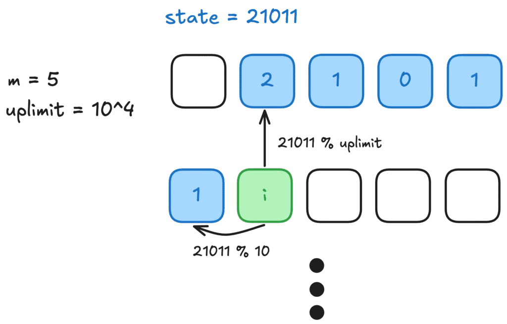
x = curr / M(row index)y = curr % M(column index)
Then use state / upLimit to get the color from the cell above, and state % 10 to get the color from the cell to the left. These checks enforce the adjacency rule at every step.
An essential component of this logic is how we build the next state. Since our state variable is an integer encoding the vertical slice of the grid, we simulate a digit shift with:
int nextState(int prev, int added) {
    return (prev % upLimit) * 10 + added;
}
This operation drops the top digit (the oldest color in the column), shifts the remaining digits to the left, and appends the new color to the end. This way, we maintain only the most recent m colors in a compact form. For example, suppose m = 2, and the previous state was 12 (representing colors 1 and 2 from top to bottom). If we add a new color 0, then the next state becomes (12 % 10) * 10 + 0 = 2 * 10 + 0 = 20. This now represents the colors 2 and 0.
Now, consider a more detailed example where m = 5 and the current state is 21011, representing top to bottom colors [2, 1, 0, 1, 1]. If we add color 0 for the next cell:
- First, drop the top color
2by taking21011 % 10000 = 1011 - Then shift left and add
0:1011 * 10 + 0 = 10110
So the new state becomes 10110, which represents colors [1, 0, 1, 1, 0].

Dynamic Programming with State Compression
Dynamic Programming becomes more powerful when combined with state compression, especially in grid coloring problems. The idea is to reduce the memory footprint of the state space to a manageable form by encoding relevant information (such as the last row’s color) into a single integer or string. This allows us to memoize states and avoid recomputing subproblems, dramatically reducing the time complexity.
To handle adjacency constraints efficiently, we encode the last m colors into a state integer and use that to determine if the next color choice is valid. If we avoid repeating colors with the last one above and to the left, we can ensure valid coloring.
To manage overlapping subproblems, we use memoization with dp[position][state], where position indicates the current cell and state encodes the coloring of previous cells.
This leads us to a recursive function that, for each position, tries each of the three colors and recurses only on valid configurations.
🔍 Walking Through the Algorithm (with Examples)
Let’s walk through a 2x2 grid!
We index cells like below.
(0,0) (0,1)
(1,0) (1,1)
Start at (0,0):
- Try red (0). Since there are no top or left neighbors, it’s valid.
state = 0- Move to
(0,1):- Can’t use red again. Try green (
1). state = nextState(0, 1) = 1
- Can’t use red again. Try green (
- Move to
(1,0):- The top is red (
0), try green (1). Valid. state = nextState(1, 1) = 11
- The top is red (
- Move to
(1,1):- Check top (
1) and left (1). Can’t be1, try0or2. - If
0,state = nextState(11, 0) = 10
- Check top (
This state-building step ensures we only track necessary adjacent values and eliminate invalid paths early.
In a 1x3 grid, we only worry about the left neighbor. Starting from the leftmost, we pick a color, ensure the next one isn’t the same, and repeat. Since only three colors exist and only adjacent constraints apply, the total number of valid colorings is quickly narrowed down.
🧾 Pseudocode
function colorTheGrid(m, n):
    M = m
    N = n
    upLimit = 10^(m-1)
    return dfs(0, 0)

function dfs(curr, state):
    if curr == N * M:
        return 1
    if dp[curr][state] exists:
        return dp[curr][state]

    x = curr / M
    y = curr % M
    totalWays = 0

    for color in [0,1,2]:
        if x > 0 and (state / upLimit == color): continue
        if y > 0 and (state % 10 == color): continue
        totalWays += dfs(curr+1, nextState(state, color))

    dp[curr][state] = totalWays % MOD
    return dp[curr][state]

function nextState(state, color):
    return (state % upLimit) * 10 + color
This code walks through each cell (curr), and for each, tries each of the three colors if they don’t match the color directly above or to the left. The state encodes the coloring history of a vertical slice, compressed using integer math.
💻 Full Source Code with Rich Comments
class Solution {
public:
    const int MOD = 1e9 + 7;
    int N, M, upLimit;
    unordered_map<int, int> dp[5*1000+1];  // Memoization table: dp[position][state]

    // Encodes new state by shifting and adding the new color
    int nextState(int prev, int added) {
        return (prev % upLimit) * 10 + added;
    }

    // Recursive DP function
    int func(int curr, int state) {
        if (curr == N * M) {
            return 1;  // Finished coloring all cells
        }
        if (dp[curr].count(state) > 0) return dp[curr][state];

        int ans = 0;
        int x = curr / M, y = curr % M;  // Compute current cell’s row and column

        // Try all 3 colors
        for (int i = 0; i <= 2; ++i) {
            // If not the first row, ensure different color than cell above
            if (x > 0 && state / upLimit == i) continue;
            // If not the first column, ensure different than cell to the left
            if (y > 0 && state % 10 == i) continue;

            ans += func(curr + 1, nextState(state, i));
            ans %= MOD;
        }

        return dp[curr][state] = ans;
    }

    int colorTheGrid(int m, int n) {
        M = m, N = n;
        upLimit = pow(10, m - 1);  // Used for slicing state digits
        return func(0, 0);
    }
};
📌 Summary and Key Takeaways
The key idea behind this problem is recognizing that while the grid has exponential possibilities, the constraints are local. By encoding the state of adjacent cells and using recursive dynamic programming with memoization, we reduce redundant computations and solve the problem efficiently.
This technique—stateful DP over grid paths with adjacency constraints—is powerful and often applicable in tiling, coloring, and robot-movement problems.